Modeling and Simulation of Chemical Process Systems

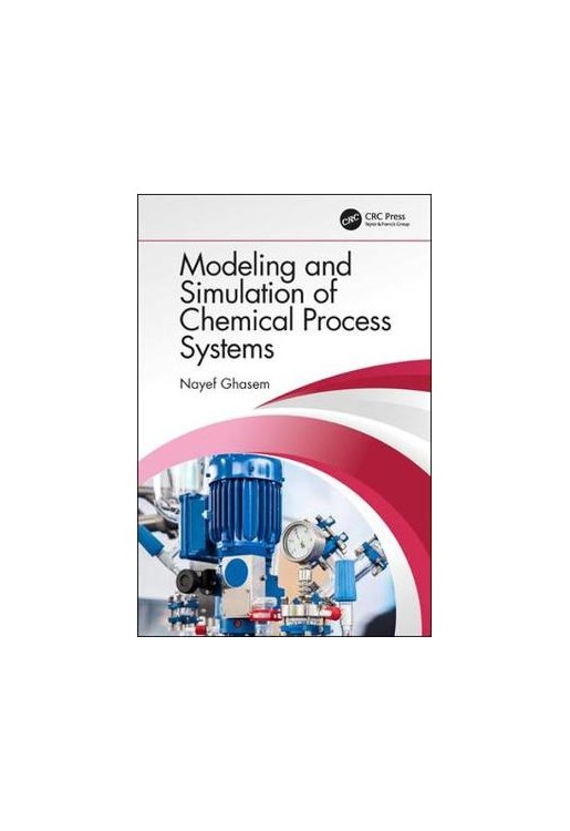
This teaches how to develop mathematical model equations, solve equations manually, and compare results with software. It covers lumped parameter systems and distributed parameter systems, and uses MATLAB and Simulink. It includes chapter problems, worked examples, and summarizes reader goals at start of every chapter.

Chapter 1: Introduction Learning objectives 1.0 Background 1.1 Mathematical models Why studying process modeling and simulation? 1.3 Terminology of process modeling and simulation 1.3.1 State variables and state equations 1.3.2 Steady state and transient 1.3.3 Lumped versus distributed parameters 1.3.4 Model verification 1.3.5 Model validation The Steps for building a mathematical model Fundamental balance equations 1.5.1 Material balance 1.5.1.1 Total and Component Balances 1.5.1.2 Material balance on individual components 1.5.2 Energy balance 1.5.3 Momentum balance 1.6 Process Classification 1.6.1 Continuous processes Batch process Semibatch Process Types of Balances Procedure of mass balance 1.8.1 Microscopic balance 1.8.2 Macroscopic balance 1.9 Transport rates 1.9.1 Mass Transport 1.9.2 Momentum transport 1.9.3 Energy transport 1.9 Thermodynamic relations 1.10 Phase Equilibrium 1.10.1 Flash calculations 1.11 Chemical kinetics Process control 1.13 Number Degree of freedom 1.14 Model solution 1.15 Model evaluation Problems References Chapter 2: Lumped Parameter Systems Learning objectives: 2.1 Introduction 2.2 Model encountered material balances only 2.2.1 Material balance without reactions 2.2.2 Material balance for chemical reactors 2.2.3 Gas phase reaction in a pressurized reactor 2.2.4 Reaction with Mass Transfer 2.3 Energy balance Problems References Chapter 3: Theory and applications of distributed systems Learning Objectives: 3.1 Introduction 3.2 Mass transport 3.2.2 Component continuity equation 3.2.2.1 Component mass continuity equation 3.2.2.2 Component molar continuity equation 3.3 Fluid dynamics 3.4 Energy transport 3.4.1 Energy transport in cartesian coordinates 3.4.2 Conversion between the coordinates 3.5 Summary of Equations of change 3.5.1 Equations of change in cartesian coordinates 3.5.2 Equations of change in Cylindrical coordinates 3.5.3 Equations of change in Spherical coordinates 3.6 Applications of the equations of change Problems References Chapter 4: Computational Fluid Dynamics Learning objectives: 4.1 Introduction 4.2 Equations of motion 4.2.1 Cartesian coordinate 4.2.2 Cylindrical coordinates 4.2.3 Spherical coordinates 4.2.4 Solving procedure 4.3 Fluid dynamic systems 4.3.1 Velocity profile in a triangular duct 4.3.2 Fluid flow in a nuzzle 4.3.3 Fluid flow past a stationary sphere 4.3.4 Incompressible fluid flows past a solid flat plate 4.4 Application to fluid dynamics Problems References Chapter 5: Mass transport of distributed systems Learning objectives. 5.1 Introduction 5.2 Diffusion of gas through membrane tube 5.3 Mass transfer with chemical reaction 5.4 Plug Flow Reactor 5.5 Diffusion of gas in solid 5.6 Diffusion with chemical reaction 5.7 Leaching of solute form solid particles 5.8 Applied examples Problems References Chapter 6: Heat transfer distributed parameter systems Learning objectives 6.1 Introduction 6.1.1 Equations of Energy 6.2 Heat Transfer from a Fin 6.3 Radial temperature gradients in an annular chemical reactor 6.4 Heat transfer in a non-Isothermal Plug-Flow reactor 6.5 Temperature profile across a composite plane wall 6.6 Applied examples Problems References Chapter 7: Case Studies Learning Objectives 7.1 Membrane reactors Equilibrium conversion 7.1.2 Numerical solution of equilibrium conversion 7.1.3 Numerical solution in case of hydrogen permeation 7.1.4 Variable feed concentration 7.1.5 Effect of membrane thickness References Absorption of Carbon dioxide from flue gas 7.2.1 Capture of carbon dioxide using fresh water 7.2.1.1 Model equations 7.2.1.2 Comsol Simulation 7.2.2 Capture of using aqueous sodium hydroxide 7.2.2.1 Model equations 7.2.2.2 Comsol Simulation References Packed bed reactors 7.3.1 Isothermal packed bed reactor 7.3.1.1 Model development 7.3.1.2 Comsol simulation 7.3.2 Adiabatic packed bed reactor References 7.4 Fluid flow of two immiscible liquids 7.4.1 Model development 7.4.2 Comsol Simulation References Production of propylene glycol in adiabatic tubular reactor 7.5.1 Model development 7.5.2 Comsol simulation References 7.6 Coupling of fluid and heat transfer (Multiphysics) 7.7 Unsteady diffusion of contaminated source from the skin of pipe line 7.8 Maxwell-Stefan diffusion 7.8.1 Hydrogen production References Chapter 8: Computing Solutions of Ordinary Differential Equations Learning objectives 8.1 Introduction 8.2 Numerical solution of single ordinary equation 8.2.1 Euler Method 8.2.2 Modified Euler's Method 8.2.3 Midpoint Method 8.2.4 Heun's Predictor Corrector Method 8.2.5 Runge-Kutta Method 8.2.5.1 Second Order Runge-Kutta 8.2.5.2 Third Order Runge-Kutta (RK3) 8.2.5.3 Fourth Order Runge-Kutta 8.3 Simultaneous Systems of first order Differential Equations Problems References Chapter 9: Higher Order Differential Equations Learning objectives 9.1 Introduction 9.2 Initial and boundary value problems 9.3 Shooting method 9.4 Simultaneous ordinary differential equation 9.5 Solving high order differential equation using Comsol Problems References